Using the Map
 The map is designed for a full computer screen; mobile functionality is restricted.
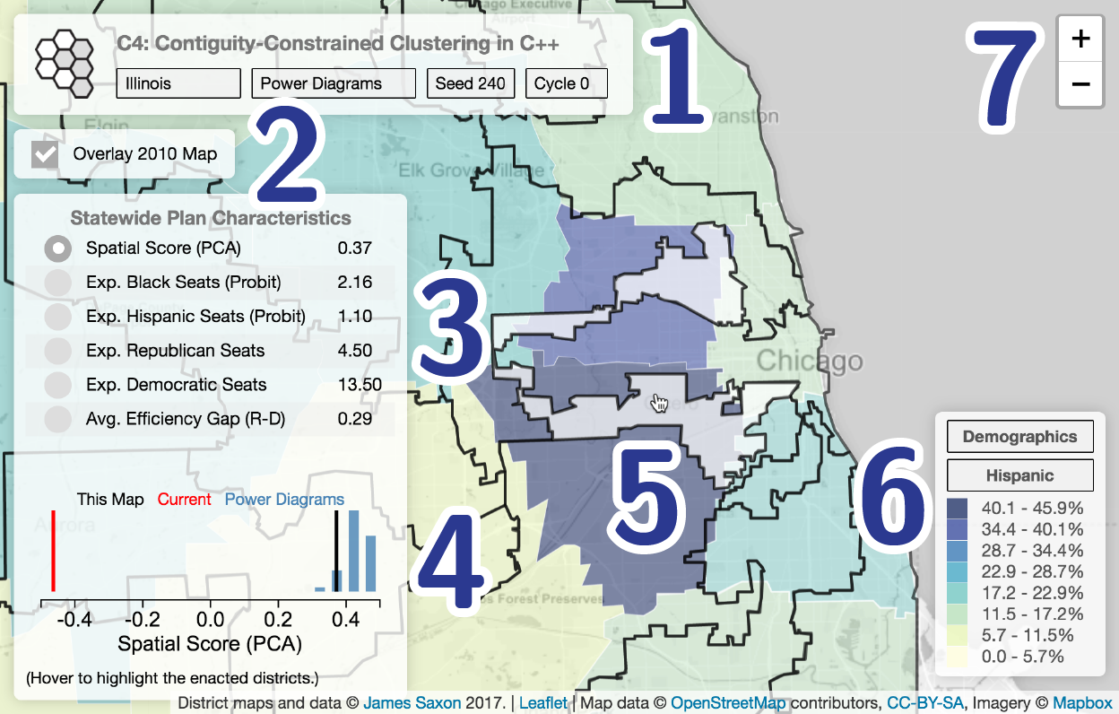
- Map Selector: Change the map shown, by state or method.
This allows the user to both put plans in a historical context, and contrast them with a non-partisan counterfactual.
The enacted maps are available for all states with multiple representatives in Congress, as are power diagrams and the single map of the split-line algorithm.
A broader variety of automated methods is available for the states with available political data (precinct-level voting returns from presidential elections): FL, IL, LA, MD, MN, NC, PA, TN, TX, VA, and WI.
The user may also select a seed or cycle to view many maps for a given state and method. This gives a sense of (a) the availability of many solutions, and (b) the quality of the maps that the given method generates. - 2010 Overlay: Toggle whether or not to show the districts of the 114th Congress, as black outlines on the map. Because the districts can still (!) be hard to make out, mousing around will highlight a single district.
- Info box: The info box presents the plan-wide characteristics: its effect on party and minority representation, and compactness. If a district is highlighted and the 2010 overlay is not activated, the box will switch to display that district's spatial characteristics.
- Map in context: Switching between characteristics in the info box, compare the selected map (black) to the enacted map from the 114th Congress, and the population of maps derived from the power diagram procedure. This shows the tradeoffs between spatial compactness, party share, and minority representation. How does the current map perform? (Party data is only available for the states listed above.)
- Highlighting districts: Moving around the map will highlight the district under the cursor. This is useful for comparing enacted districts to the currently selected basemap. If the 2010 map is not activated, it will change the info box.
- Map shading and legend:
The legend is manipulable. You can shade districts by:
- District number: This makes it easier to view boundaries.
- Population equality: Population equality is required, per Karcher v. Daggett (1983). The states aim for and often claim perfect equality based on the Census counts. But the data are not precise enough to support the claims of accuracy made, and populations change over the course of a decade between Censuses. In practice, in my methods, I have aimed for population deviations of less than 2% with respect to the target.
- Party Share: In states where detailed voting data is available, you can scan through elections, and estimate who would have won the districts currently mapped, based on presidential votes.
- Demographics: Understand the spatial distribution of black and hispanic minorities in a state. This is important for understand impacts on minority representation. Intentional "minority districts" stand out on many of the enacted maps.
- Compactness: Of course, you can display the spatial characteristics of a plan! Consult the paper for a description of each of the methods.
- Zoom to home: Switching states will automatically center that state in the window. But the maps is fully manipulable. Zoom and pan to view your home or investigate other details of maps.
Scoring Plans: Probits, PCAs, and Aggregated Votes...
Expected minority representation is based on a probit model that regresses minority representation on the black and hispanic share of the voting age population (VAP) in each congressional district of the 115th Congress. For non-experts: a "probit model" just means that I am modelling the probability of getting a minority representative.
Expected party share is calculated by aggregating votes cast at the precinct level in Presidential general elections, within the boundaries of simulated or enacted districts. (A point in polygon merge is used.) The quoted seat share is the average over the available elections. For historic maps where states' delegations may have had a different size, the share accruing to parties and minorities are rescaled to the 2010 baseline.
Spatial scores come from the first principal component of the many compactness definitions, evaluated on the population of enacted maps used for the 107th, 111th, and 114th Congresses (1990, 2000, and 2010 Censuses). A "principle component analysis" (PCA) is a fancy way of reducing a many different properties of a collection of objects to fewer variables, while preserving information (dimensionality reduction). The "first component" contains as much of the variation as possible of real districts' compactness scores in a single measure. The "second component" takes as much as possible of the variance that remains after the first component, and so forth.
Data Sources
Populations, demographics (race and ethnicity), and geographies (congressional districts, census tracts, block groups, blocks, and voter tabulation districts) are from the US Census. Simulations use the American Community Survey 5-year estimates, and the historical districts are based on the appropriate decennial Census. The geographies are through TIGER. Census tract edges are simplified for simulation. Simulations and map data are through the C4 package, and are copyright James Saxon 2017.
The precinct level returns are assembled from many sources. Florida (2008) and Illinois (2008) are by Ansolabehere et al. (2011) Maryland (2008) Pennsylvania (2000-2012) and Texas (1996-2012) use election returns by Ansolabehere, et al. (2015) merged with Voter Tabulation Districts (VTDs) from the Census (2010) and precincts and additional voting data from Texas (2012, 2016). For Pennsylvania in 2012, the precinct names were slightly inconsistent; and a number of manual corrections and fuzzy matches were required. I supplement the Pennsylvania and Texas returns with data directly from the states for Louisiana (2012, 2016: votes and maps), Illinois (2016 votes), Maryland (2016 votes), Minnesota (2008-2016), North Carolina (2012, 2016: votes and maps), Tennessee (2016 votes and maps), Virginia (2016), and Wisconsin (2004-2016).
For the geographies, there are several special cases. For Maryland in 2016, the polling places and not precincts were available; I therefore use the former. The Virginia shapefiles are courtesy of the Virginia Public Access Project (2017), with some corrections (duplicated layers, and an update for Roanoke City). The Illinois precincts have changed significantly since the 2010 Census release, and I have updated Cook (Chicago and rest), DuPage, and Lake Counties. Together, these cover most of the changes and more than half of the state’s population. The rest of the state is matched by precinct and county name. In cases like North Carolina where early, absentee, and provisional voting are recorded at the county level, I divide these votes among precincts in proportions equal to the polling-place share of the county vote for each party.
These mapped data are available upon request, with attribution.